what is the electron charge to masss ratio used in

APPARATUS

• Kent \(due east/grand\) Experimental Apparatus Model TG-xiii
• GW Laboratory DC Power Supply Model GPS-1850
• Heathkit Regulated Power Supply Model PS-four
• Triplett Multimeter Model 4000
• Simpson Digital Multimeter Model 464
• Bell 620 Gaussmeter with Hall Probe
• Magnetic compass

INTRODUCTION

Measuring separately the electric charge (\(e\)) and the residue mass (\(grand\)) of an electron is a hard task because both quantities are extremely small (\(e\) = 1.60217733×10^-19 coulombs, \(thou\) = nine.1093897×x^-31 kilograms). Fortunately, the ratio of these two fundamental constants can exist determined hands and precisely from the radius of curvature of an electron beam traveling in a known magnetic field. An electron beam of a specified free energy, and therefore a specified speed, may exist produced conveniently in an \(e/m\) apparatus. The central piece of this apparatus is an evacuated electron-beam bulb with a special anode. A known current flows through a pair of Helmholtz coils and produces a magnetic field. The trajectory of the speeding electrons moving through the magnetic field is made visible past a small amount of mercury vapor.

THEORY

An electron moving in a uniform magnetic field travels in a helical path effectually the field lines. The electron's equation of motion is given by the Lorentz relation. If in that location is no electric field, then this relation can be written as

\begin{eqnarray} \textbf{F}_B &=& -due east(\textbf{v}\times\textbf{B}), \label{eqn_1} \end{eqnarray}

where \(\textbf{F}_B\) is the magnetic force on the electron, \(-e\) = -one.6×10^-xix coulombs is the electric charge of the electron, \(v\) is the velocity of the electron, and \(\textbf{B}\) is the magnetic field. In the special case where the electron moves in an orbit perpendicular to the magnetic field, the helical path becomes a circular path, and the magnitude of the magnetic force is

\begin{eqnarray} F_B &=& evB. \label{eqn_2} \terminate{eqnarray}

Recall from Physics 6A that an object traveling around a circle experiences a centripetal force. For an electron of mass g moving at speed \(v\) in a circle of radius \(R\), the magnitude of the centripetal force \(F_C\) is

\brainstorm{eqnarray} F_C &=& mv^two/R. \label{eqn_3} \end{eqnarray}

Therefore,

\brainstorm{eqnarray} evB &=& mv^ii /R, \end{eqnarray}

or

\begin{eqnarray} eB &=& mv/R. \characterization{eqn_4} \stop{eqnarray}

The initial potential free energy of the electrons in this experiment is \(eV\), where \(V\) is the accelerating voltage used in the electron-axle tube. After the electrons are accelerated through a voltage \(V\), this initial potential energy is converted into kinetic free energy \((i/2)mv^2\). Since energy is conserved, it follows that

\begin{eqnarray} eV &=& (1/ii)mv^ii. \characterization{eqn_5} \cease{eqnarray}

Combining Eqs. 4 and 5 yields

\begin{eqnarray} eastward/m &=& 2V/B^2 R^two. \label{eqn_6} \terminate{eqnarray}

THE \(e/m\) APPARATUS

The electron-axle bulb used in this experiment has a cathode that is heated indirectly, a collimating filigree with a pigsty, and an anode with a pigsty.

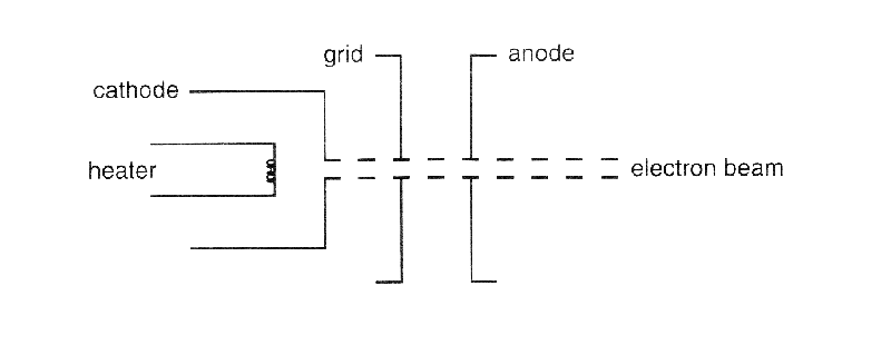
Electrons leave the heated cathode and are attracted by the anode, which has a positive potential with respect to the cathode. Most electrons are stopped by the collimating grid and the anode. Those that are able to laissez passer through the pigsty in the anode emerge from the back of the anode equally a thin, monochromatic beam. The kinetic energy of the electrons in this beam is equal to the potential energy departure between the anode and the cathode.

To make the path of the electrons visible, we apply the following method. The large evacuated glass bulb that houses the cathode and anode is spiked with a trace of mercury, enough to produce nearly saturated mercury vapor with a pocket-sized pressure of approximately 1×10^-3 mm Hg. (By comparison, recall that normal temper pressure is approximately 760 mm Hg.) Occasionally an electron from the beam with a kinetic energy of about 300 eV collides with a mercury cantlet, causing the cantlet to get excited — a procedure that requires 10.4 eV of energy. The excited cantlet then decays quickly back to the footing state, emitting several photons in the procedure (including the one that has the feature blue color of mercury calorie-free). Thus, the blue halo in the glass bulb marks the path of the electrons. Notation that the electron-beam tube, forth with its socket, can be rotated well-nigh ninety°.

The Helmholtz coils consist of a pair of identical circular coils of wire, each of radius \(r\), connected in series.

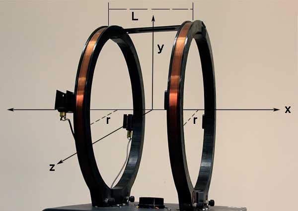
The distance between the coils is denoted \(L\). When \(L \ll r\), the coils produce a nearly uniform magnetic field in the space between them.

Forth the centrality of ane thin coil with \(North\) turns at a distance \(x\) from the airplane of the curl, the magnitude of the magnetic field \(B\) due to a current \(I\) is

\begin{eqnarray} B &=& \mu_0 r^2 Northward I/[2(r^two+ten^ii)^{3/2}]. \label{eqn_7} \end{eqnarray}

The direction of the magnetic field is perpendicular to the airplane of the roll, and its unit is the tesla (T), with 1 tesla = 10⁴ gauss. In SI units, the magnetic permeability μ₀ of free space is

\begin{eqnarray} \mu_0 &=& 4\pi\times 10^{-seven} \textrm{ Tm/A}. \end{eqnarray}

For a pair of identical parallel coils separated by a distance \(L\), the magnitude of the magnetic field at a point along the \(x\)-axis is

\brainstorm{eqnarray} B &=& [\mu_0 r^2 NI/2] [ one/(r^ii+x^two)^{three/2} + 1/(r^two+(L-x)^2)^{3/2} ]. \label{eqn_8} \cease{eqnarray}

When \(x = L/ii \), Eq. \eqref{eqn_8} gives

\begin{eqnarray} B &=& \mu_0 r^ii NI/(r^ii+L^2/4)^{3/ii}. \label{eqn_9} \cease{eqnarray}

EQUIPMENT

The centerpiece of this experiment is the Kent \(due east/m\) Experimental Apparatus Model TG-xiii, which consists of the electron-beam bulb (EBB) and a pair of Helmholtz coils (HC). There is too an illuminated ruler behind the EBB to facilitate the measurement of the electron-beam radius. The apparatus is fed by three external power sources. The accelerating voltage for the EBB is produced by a Heathkit Regulated Power Supply Model PS-4. A voltage of 150 – 300 5 at a modest current of approximately 50 mA is required. This supply too provides the cathode heater power using a 6.three-Five alternating current. The electrical current and voltages are measured with two digital multimeters: the Triplett Multimeter Model 4000 and Simpson Digital Multimeter Model 464.

We use a GW Laboratory DC Power Supply Model GPS-1850 for the HC, which as well supplies the voltage for the small low-cal bulb of the illuminated scale. A large current of 1 – 2 A is needed, but a low voltage of v – xv 5 is adequate. The \(eastward/m\) apparatus may be covered with a blackness cloth to reduce background light.

INITIAL SETUP

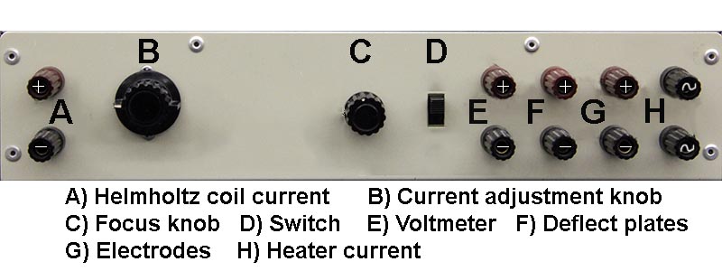
On the front panel of the \(e/yard\) appliance are jacks for the power and the voltmeter, two control knobs, and a switch. Starting from the left side of the console, nosotros have:

1. 2 jacks (A) for the connection to the Helmholtz coils (HC) power supply. The current is measured by a multimeter connected in series with the power supply.

2. A electric current adjustment knob (B) for the HC. (The electric current can also be changed directly past a knob on the power supply.)

3. The focus knob (C), which allows sharpening of the electron axle past variation of the voltage on the grid of the EBB. The grid is internally connected and does not need a separate power supply.

4. A switch (D). This should exist set in the "e/m Measure" position.

5. Ii jacks (Due east) for the voltmeter, which measures the accelerating voltage.

6. 2 jacks (F) for the deflection plates. (These are not used.)

7. Two jacks (G) for the loftier-voltage (~300 V) input to the electrodes of the electron gun.

8. Two jacks (H) for connecting the electron-gun heater to the power supply which can be 6.iii-5 DC or Ac. (We use AC.)

Connect the EBB to the power supplies and multimeters (see the figure below).

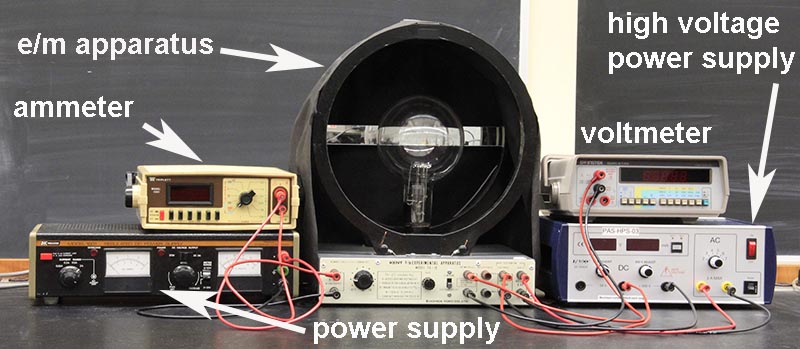
Utilise red cables for positive voltage and black cables for ground. To measure the HC electric current, make sure information technology passes through the Triplett multimeter in the current style. (The HC power supply, the ammeter, and the HC are therefore continued in series.) Plug in the ability supplies and the multimeters. Prepare the Triplett multimeter to the highest current scale, and put it in the DC-A mode. Connect the Simpson multimeter to the jacks labeled for the voltmeter (item Eastward on the front panel of the EBB) ready to the highest voltage calibration, and put it in the DC-V manner.

Procedure

1. Orient the Helmholtz coils (HC) so as to eliminate the influence of the World's magnetic field on the experiment. To do this, employ a magnetic compass to decide the direction of the Earth's field, marking its management on your piece of work station with paper tape, and record its coordinates. As well measure and record the dip bending. Rotate the coils such that the plane of the HC lies in the plane of the Earth's magnetic field. With this orientation, the issue of the Earth's field on the HC is zero.

2. Connect the power supplies and multimeters to the \(eastward/one thousand\) apparatus, as detailed in the previous section. Cheque that the polarities agree with the ones marked on the front end panel of the appliance.

3. Identify the black cloth over the HC for piece of cake observation of the electron beam. Plough on the heater supply, and allow 2 minutes for the filament to heat up. Apply 150 V to the anode, which should produce a visible beam. Turn on the current through the HC, and observe how the electron beam is aptitude and forms a circle.

4. Very advisedly, rotate the glass bulb and observe the helical path of the electrons. Notice the direction of the helical axis.

5. Rotate the glass bulb such that the aeroplane of the electron beam is exactly parallel to the aeroplane of the HC. Using the focus control, obtain a well-divers beam. (You may also demand to adjust the filament power to accomplish this.) If necessary, make a fine aligning of the EBB's orientation so that the axle, after traveling a full circumvolve, passes between the two metal struts which feed the power to the filament.

6. Ready the HC current at a fixed value (e.g., 1 A). Measure out \(R\) (the radius of the electron axle) for at least 4 settings of \(V\) (the accelerating voltage). Since \(east/m\) is proportional to \(ane/R^2\), you lot should make an endeavour to measure \(R\) with small uncertainty. Use the mirror backside the EBB to minimize parallax. You may add a 2nd ruler that is taped to the front of the HC.

7. Prepare the accelerating voltage at a fixed value (e.g., 200 V). Measure \(R\) for at least four settings of \(I\) (the HC current).

   The manufacturer of the \(e/m\) apparatus did not supply the number of windings, \(N\), of the HC. On the forepart console of the EBB stand, it is stated that \(B\) = (7.8 \(I\)) gauss, simply no incertitude is given. To determine the magnitude of the magnetic field, you volition use a calibrated magnetometer (Bong 620 Gaussmeter) based on a calibrated Hall Probe.

   Your TA will remove the EBB. Install the Hall-Probe holder in the HC. Calibrate the magnitude of the magnetic field \(B\) in the center of the HC for the four values of the current \(I\), including two dissimilar scale settings. Plot \(B\) as a function of \(I\). Note that the error in \(east/1000\) is proportional to \(1/B^2\) (come across Eq. \eqref{eqn_6}). Utilise the \(B\) versus \(I\) graph to determine the magnetic field for each value of the current.

8. Plot \(V\) equally a function of \(R^2\) (the data in pace half-dozen), and use the slope of the graph to determine the ratio \(e/m\) with the assistance of Eq. \eqref{eqn_6}.

9. Plot \(I^2\) as a function of \(i/R^two\) (the data in step 7), and utilise the slope of the graph to determine the ratio \(east/one thousand\) with the help of Eq. \eqref{eqn_6}.

10. Compute the ratio \(e/thou\) using the "accepted" values provided in the "Introduction" department of this experiment, and compare information technology with your measured ratios from parts eight and 9.

Decision OF THE Acceleration VOLTAGE

The absolute scale of a voltage meter is a very hard task. Traditionally, 1 uses standard cells which are stored at the National Scale Laboratory in various countries. A new method depends on the and then-called Josephson consequence. Nosotros will presume that the multimeters have been calibrated sufficiently well. Still, we should compare the voltage readings of the two multimeters to estimate the minimal value for the absolute error.

DATA

1. Coordinates of Earth's magnetic field =

   Dip angle =

6. \(V\) (Trial 1) =

   \(R\) (Trial 1) =

   \(V\) (Trial 2) =

   \(R\) (Trial two) =

   \(Five\) (Trial 3) =

   \(R\) (Trial three) =

   \(V\) (Trial 4) =

   \(R\) (Trial 4) =

7. \(I\) (Trial one) =

   \(R\) (Trial i) =

   \(I\) (Trial ii) =

   \(R\) (Trial two) =

   \(I\) (Trial 3) =

   \(R\) (Trial iii) =

   \(I\) (Trial 4) =

   \(R\) (Trial 4) =

   \(B\) (Trial ane) =

   \(B\) (Trial ii) =

   \(B\) (Trial three) =

   \(B\) (Trial iv) =

   Plot the graph of \(B\) as a function of \(I\) using one sheet of graph paper at the finish of this workbook. Recollect to label the axes and title the graph.

8. Plot the graph of \(V\) every bit a office of \(R^2\) using one sheet of graph paper at the end of this workbook. Remember to characterization the axes and title the graph.

   Gradient of graph =

   \(eastward/m\) =

9. Plot the graph of \(I^2\) as a function of \(1/R^two\) using ane canvas of graph paper at the end of this workbook. Call up to label the axes and title the graph.

   Slope of graph =

   \(e/k\) =

10. \(due east/m\) (computed from accustomed values provided in "Introduction") =

    Pct divergence between experimental and accepted \(e/m\) from role 8 =

    Per centum difference between experimental and accustomed \(e/chiliad\) from part ix =

velezanscialtat.blogspot.com

Source: https://demoweb.physics.ucla.edu/content/experiment-6-charge-mass-ratio-electron

Share this post